O(1) or constant time complexity.O(n^2), where n is the size of the list to be sorted.O(n*log(n)), where n is the size of the list to be sorted.
1x1 square on its own. If a field has free fields on its left, top, and top-left, then it’s the bottom-right corner of a 2x2 square. If those three fields are all bottom-right corners of a 5x5 square, then their overlap, plus the queried field being free, form a 6x6 square. We can use this logic to solve this problem. That is, we define the relation of size[x, y] = min(size[x-1, y], size[x, y-1], size[x-1, y-1]) + 1 for every free field. For an occupied field, we can set size[x,y] = 0, and it will fit our recursive relation perfectly. Now, size[x, y] represents the largest square for which the field is the bottom-right corner. Tracking the maximum number achieved will give us the answer to our problem.FUNCTION square_size(board)
M = board.height()
N = board.width()
size = Matrix[M + 1, N + 1]
FOR i IN [0..M]
size[i, 0] = 0
END FOR
FOR i IN [0..N]
size[0, i] = 0
END FOR
answer = 0
FOR i IN [0..M]
FOR j IN [0..N]
size[i+1, j+1] = max(size[i, j+1], size[i+1, j], size[i, j]) + 1
answer = max(answer, size[i+1, j+1])
END FOR
END FOR
RETURN answerCiphertext”. To convert the text, algorithm uses a string of bits referred as “keys” for calculations. The larger the key, the greater the number of potential patterns for creating cipher text. Most encryption algorithm use codes fixed blocks of input that have length about 64 to 128 bits, while some uses stream method. a = a + b;
b = a - b; // this will act like (a+b) - b, and now b equals a.
a = a - b; // this will act like (a+b) - a, and now an equals b.Integer.MAX_VALUE in Java, or if the subtraction is less than the minimum value of the int primitive type as defined by Integer.MIN_VALUE in Java, there will be an integer overflow.XOR method. This is often regarded as the best approach because it works in languages that do not handle integer overflows, such as Java, C, and C++. Java has a number of bitwise operators. XOR (denoted by ^) is one of them.x = x ^ y;
y = x ^ y;
x = x ^ y;i and j(string)-1, to set J at last positionstring [0], to set i on the first character.string [i] is interchanged with string[j]i>j then go to step3(72538) -> (27538) swap 7 and 2.
(27538) -> (25738) swap 7 and 5.
(25738) -> (25378) swap 7 and 3.
(25378) -> (25378) algorithm does not swap 7 and 8 because 7<8.(25378) -> (25378) algorithm does not swap 2 and 5 because 2<5.
(25378) -> (23578) swap 3 and 5.
(23578) -> (23578) algorithm does not swap 5 and 7 because 5<7.
(23578) -> (23578) algorithm does not swap 7 and 8 because 7<8.
New_node-> Next= head;
Head=New_node While( P!= insert position)
{
P= p-> Next;
}
Store_next=p->Next;
P->Next= New_node;
New_Node->Next = Store_next; While (P->next!= null)
{
P= P->Next;
}
P->Next = New_Node;
New_Node->Next = null; T = ∅;
U = { 1 };
while (U ≠ V)
let (u, v) be the lowest cost edge such that u ∈ U and v ∈ V - U;
T = T ∪ {(u, v)}
U = U ∪ {v}KRUSKAL(G):
A = ∅
For each vertex v ∈ G.V:
MAKE-SET(v)
For each edge (u, v) ∈ G.E ordered by increasing order by weight(u, v):
if FIND-SET(u) ≠ FIND-SET(v):
A = A ∪ {(u, v)}
UNION(u, v)
return AB -> D of the shortest path A -> D between vertices A and D is also the shortest path between vertices B and D.
function dijkstra(G, S)
    for each vertex V in G
        distance[V] <- infinite
        previous[V] <- NULL
        If V != S, add V to Priority Queue Q
    distance[S] <- 0

    while Q IS NOT EMPTY
        U <- Extract MIN from Q
        for each unvisited neighbour V of U
            tempDistance <- distance[U] + edge_weight(U, V)
            if tempDistance < distance[V]
                distance[V] <- tempDistance
                previous[V] <- U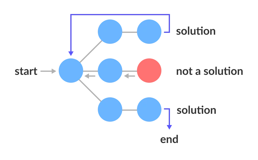
return distance[], previous[]Backtrack(x)
if x is not a solution
return false
if x is a new solution
add to list of solutions
backtrack(expand x)
FUNCTION find_anagrams(words)
    word_groups = HashTable<String, List>
    FOR word IN words
        word_groups.get_or_default(sort(word), []).push(word)
    END FOR
    anagrams = List
    FOR key, value IN word_groups
        anagrams.push(value)
    END FOR
RETURN anagrams ​status=1 (ready state) status=2, i.e. (waiting state)status=3, i.e. (processed state)state (status=1) and set their status =2 (waiting state)dictionary[] = {"FREE", "TIME", "LEARN"};
boggle[][] = {{'F', 'A', 'R'},
{'E', 'R', 'E'},
{'L', 'I', 'E'}};
isWord(str): returns true if str is present in dictionary
else false.buildMaxHeap() function. This function, also known as heapify(), creates a heap from a list in O(n) operations.siftDown() function on the list.buildMaxHeap() operation runs only one time with a linear time complexity or O(n) time complexity. The siftDown() function works in O(log n) time complexity, and is called n times. Therefore, the overall time complexity of the heap sort algorithm is O(n + n log (n)) = O(n log n).delNode(). In a direct implementation, the function needs to adjust the head pointer when the node to be deleted the first node.#include <stdio.h>
#include <stdlib.h>
struct Node
{
int data;
struct Node *next;
};
void delNode(struct Node *head, struct Node *n)
{
if(head == n)
{
if(head->next == NULL)
{
printf("list can't be made empty because there is only one node. ");
return;
}
head->data = head->next->data;
n = head->next;
head->next = head->next->next;
free(n);
return;
}
struct Node *prev = head;
while(prev->next != NULL && prev->next != n)
prev = prev->next;
if(prev->next == NULL)
{
printf("\n This node is not present in List");
return;
}
prev->next = prev->next->next;
free(n);
return;
}
void push(struct Node **head_ref, int new_data)
{
struct Node *new_node =
(struct Node *)malloc(sizeof(struct Node));
new_node->data = new_data;
new_node->next = *head_ref;
*head_ref = new_node;
}
void printList(struct Node *head)
{
while(head!=NULL)
{
printf("%d ",head->data);
head=head->next;
}
printf("\n");
}
int main()
{
struct Node *head = NULL;
push(&head,3);
push(&head,2);
push(&head,6);
push(&head,5);
push(&head,11);
push(&head,10);
push(&head,15);
push(&head,12);
printf("Available Link list: ");
printList(head);
printf("\nDelete node %d: ", head->next->next->data);
delNode(head, head->next->next);
printf("\nUpdated Linked List: ");
printList(head);
/* Let us delete the the first node */
printf("\nDelete first node ");
delNode(head, head);
printf("\nUpdated Linked List: ");
printList(head);
getchar();
return 0;
}​Available Link List: 12 15 10 11 5 6 2 3
Delete node 10:
Updated Linked List: 12 15 11 5 6 2 3
Delete first node
Updated Linked list: 15 11 5 6 2 3 1->2->3 and second is 12->10->2->4->6, the first list should become 1->12->2->10->17->3->2->4->6 and second list should become empty. The nodes of the second list should only be inserted when there are positions available.O(n) where n is number of nodes in first list.#include <stdio.h>
#include <stdlib.h>
struct Node
{
int data;
struct Node *next;
};
void push(struct Node ** head_ref, int new_data)
{
struct Node* new_node =
(struct Node*) malloc(sizeof(struct Node));
new_node->data = new_data;
new_node->next = (*head_ref);
(*head_ref) = new_node;
}
void printList(struct Node *head)
{
struct Node *temp = head;
while (temp != NULL)
{
printf("%d ", temp->data);
temp = temp->next;
}
printf("\n");
}
void merge(struct Node *p, struct Node **q)
{
struct Node *p_curr = p, *q_curr = *q;
struct Node *p_next, *q_next;
while (p_curr != NULL && q_curr != NULL)
{
p_next = p_curr->next;
q_next = q_curr->next;
q_curr->next = p_next;
p_curr->next = q_curr;
p_curr = p_next;
q_curr = q_next;
}
*q = q_curr;
}
int main()
{
struct Node *p = NULL, *q = NULL;
push(&p, 3);
push(&p, 2);
push(&p, 1);
printf("I Linked List:\n");
printList(p);
push(&q, 8);
push(&q, 7);
push(&q, 6);
push(&q, 5);
push(&q, 4);
printf("II Linked List:\n");
printList(q);
merge(p, &q);
printf("Updated I Linked List:\n");
printList(p);
printf("Updated II Linked List:\n");
printList(q);
getchar();
return 0;
} ​I Linked List:
1 2 3
II Linked List:
4 5 6 7 8
Updated I Linked List:
1 4 2 5 3 6
Updated II Linked List:
7 8