Google News
logo
TensorFlow.js Interview Questions
TensorFlow.js is a JavaScript Library for training and deploying "machine learning" models in the browser and in Node.js. Tensorflow lets us add machine learning functions to any Web Application.
 
Developed in 2015 by the Google Brain Team, it ensures to provide an easy-to-use low-level toolkit that can handle complex mathematical operations and learning architectures.
 
TensorFlow can be used in a wide variety of programming languages, most notably Python, as well as Javascript, C++, and Java. This flexibility lends itself to a range of applications in many different sectors.
Prerequisite : Before starting Tensorflow.js, you need to know the following :
 
For browser :
 
* HTML : Basics knowledge of HTML is required
* JavaScript : Good knowledge of JS is required
 
 
For server-side :
 
* Node.js : Having a good command of Node.js. Also since Node.js is a JS runtime, so having command over JavaScript would help a lot.


Other requirements :
 
* NPM or Yarn : These are packages that need to be installed in your system.
There are two main ways to get TensorFlow.js in your browser based projects:
 
* Using script tags.
 
* Installation from NPM and using a build tool like Parcel, WebPack, or Rollup.
 
If you are new to web development, or have never heard of tools like webpack or parcel, we recommend you use the script tag approach. If you are more experienced or want to write larger programs it might be worthwhile to explore using build tools.
 
Usage via Script Tag : Add the following script tag to your main HTML file.
<script src="https://cdn.jsdelivr.net/npm/@tensorflow/tfjs@2.0.0/dist/tf.min.js"></script>
See code sample for script tag setup
// Define a model for linear regression.
const model = tf.sequential();
model.add(tf.layers.dense({units: 1, inputShape: [1]}));

model.compile({loss: 'meanSquaredError', optimizer: 'sgd'});

// Generate some synthetic data for training.
const xs = tf.tensor2d([1, 2, 3, 4], [4, 1]);
const ys = tf.tensor2d([1, 3, 5, 7], [4, 1]);

// Train the model using the data.
model.fit(xs, ys, {epochs: 10}).then(() => {
  // Use the model to do inference on a data point the model hasn't seen before:
  model.predict(tf.tensor2d([5], [1, 1])).print();
  // Open the browser devtools to see the output
});
  
Installation from NPM : You can use either the npm cli tool or yarn to install TensorFlow.js.
yarn add @tensorflow/tfjs
or
npm install @tensorflow/tfjs
See sample code for installation via NPM
import * as tf from '@tensorflow/tfjs';

// Define a model for linear regression.
const model = tf.sequential();
model.add(tf.layers.dense({units: 1, inputShape: [1]}));

model.compile({loss: 'meanSquaredError', optimizer: 'sgd'});

// Generate some synthetic data for training.
const xs = tf.tensor2d([1, 2, 3, 4], [4, 1]);
const ys = tf.tensor2d([1, 3, 5, 7], [4, 1]);

// Train the model using the data.
model.fit(xs, ys, {epochs: 10}).then(() => {
  // Use the model to do inference on a data point the model hasn't seen before:
  model.predict(tf.tensor2d([5], [1, 1])).print();
  // Open the browser devtools to see the output
});
  
Node.js Setup : You can use either the npm cli tool or yarn to install TensorFlow.js.
 
Option 1 : Install TensorFlow.js with native C++ bindings.
yarn add @tensorflow/tfjs-node
or
npm install @tensorflow/tfjs-node
Option 2 : (Linux Only) If your system has a NVIDIA® GPU with CUDA support, use the GPU package even for higher performance.
yarn add @tensorflow/tfjs-node-gpu
or
npm install @tensorflow/tfjs-node-gpu
Option 3 : Install the pure JavaScript version. This is the slowest option performance wise.
yarn add @tensorflow/tfjs
or
npm install @tensorflow/tfjs
See sample code for Node.js usage
const tf = require('@tensorflow/tfjs');

// Optional Load the binding:
// Use '@tensorflow/tfjs-node-gpu' if running with GPU.
require('@tensorflow/tfjs-node');

// Train a simple model:
const model = tf.sequential();
model.add(tf.layers.dense({units: 100, activation: 'relu', inputShape: [10]}));
model.add(tf.layers.dense({units: 1, activation: 'linear'}));
model.compile({optimizer: 'sgd', loss: 'meanSquaredError'});

const xs = tf.randomNormal([100, 10]);
const ys = tf.randomNormal([100, 1]);

model.fit(xs, ys, {
  epochs: 100,
  callbacks: {
    onEpochEnd: (epoch, log) => console.log(`Epoch ${epoch}: loss = ${log.loss}`)
  }
});


Source : Tensorflow

Tensors are similar to arrays in programming languages, but here, they are of higher dimensions. It can be considered as a generalization of matrices that form an n-dimensional array. TensorFlow provides methods that can be used to create tensor functions and compute their derivatives easily. This is what sets tensors apart from the NumPy arrays.
TensorBoard is a Graphical User Interface (GUI) that is provided by TensorFlow to help users visualize graphs, plots, and other metrics easily without having to write a lot of code. TensorBoard provides an ample number of advantages in terms of readability, ease of use, and performance metrics.
There are three types of Tensors used to create neural network models:
 
Constant Tensor : Constant Tensors are used as constants, as the name suggests. They create a node that takes a value and does not change it. A constant can be created using tf.constant.
tf.constant(value, dtype=None, shape=None, name='Const', verify_shape=False)
It accepts the five arguments.

Variable Tensor : Variable Tensors are the nodes which provide their current value as output. It means that they can retain their value over multiple executions of a graph.

Place Holder Tensor : Placeholders Tensors are essential than variables. These are used to assign data in a later time. Placeholders are the nodes whose value is fed at the time of execution. Assume, we have inputs to our network which are dependent on some external data. Also, we do not want our graph to depend on any real value while developing the graph, then Placeholders are useful datatype. We can even build a graph without any data.

Therefore, placeholders do not require any initial value. They only need a datatype (such as float32) and a tensor shape, so the graph still knows what to compute with even though it does not have any stored values.
Tensorflow has APIs support for a wide variety of languages such as Matlab and C++. Researchers are continuously trying to making it better. A javascript library, tensorflow.js, has also been introduced for training and deploying machine learning models.
TensorFlow has numerous advantages, and this is why it is the most used framework for Machine Learning in the world. Some of its advantages are given below:
 
* Platform independency
* Auto-differentiation capability
* Open-source and large community
* Support for asynchronous computations
* Usage of GPU for distributed computing
* Highly customizable based on requirements
TensorFlow has some limitations, as mentioned here :
 
* It does not provide support for OpenCL (Open Computing Language).
* It requires prior knowledge of advanced calculus and linear algebra along with a pretty good understanding of Machine learning.
* It has GPU memory conflicts with Theano if imported in the same scope.
It is the central unit in the architecture of TensorFlow Serving, which serves as objects used by the clients in the process of computations. It offers flexible size and granularity. It consists of one lookup table to a tuple of interference models.
 
Typical servables include the following :

* a TensorFlow SavedModelBundle (tensorflow::Session)
* a lookup table for embedding or vocabulary lookups
 
It improves the functionality and performance with the help of improvements:
 
* streaming results
* experimental APIs
* asynchronous modes of operation

TensorFlow serving allows the system of TensorFlow, which we use for machine learning. It allows us to create, use, and execute the algorithms for the system a user wants to build. It extends its functionality with the help of collaborating environments such as TensorBoard.
Tensorflow Loaders are used for adding algorithms and data backends one of which is tensorflow itself. For example, a loader can be implemented to load, access and unload a new type of servable machine learning model.
TensorFlow provides support for multiple client languages, one of the best among them is Python. There are some experimental interfaces which are available for C++, Java, and Go. A language bindings for many other languages such as C#, Julia, Ruby, and Scala are created and supported by the open-source community.
There are two ways that you can use to load data into TensorFlow before training Machine Learning algorithms :
 
Data load into memory : Here, the data is loaded into the memory as a single array unit. It is the easiest way to load the data.

TensorFlow data pipeline : It is making use of the built-in APIs to load the data and feed it across to the algorithm.
There are five main steps that govern the working of the majority of algorithms in TensorFlow. They are as follows:
 
* Data import or data generation, alongside setting up a data pipeline
* Data input through computational graphs
* Generation of the loss function to evaluate the output
* Backpropagation to modify the data
* Iterating until output criteria are met
* Import data, generate data, or setting a data-pipeline through placeholders.
* Feed the data through the computational graph.
* Evaluate output on the loss function.
* Use backpropagation to modify the variables.
* Repeat until stopping condition.
* Dropout Technique
* Regularization
* Batch Normalization
The TensorFlow managers are responsible for loading, unloading, lookup, and lifetime management of all servable objects via their loaders. TensorFlow Managers control the full lifecycle of Servables, including :
 
* Loading Servables
* Serving Servables
* Unloading Servables

It is an abstract class. Its syntax is :
#include <manager.h>  
TensorFlow is used in all of the domains that cover Machine Learning and Deep Learning. Being the most essential tool, the following are some of the main use cases of TensorFlow:
 
* Voice recognition
* Video upscaling
* Image recognition
* Test-based applications
* Time series analysis
Python is the primary language when it comes to working with TensorFlow. TensorFlow provides ample number of functionalities when used with the API, such as :
 
* Automatic logging
* Automatic checkpoints
* Simple training distribution
* Queue-runner design methods
Following are some of the APIs developed by Machine Learning enthusiasts across the globe :
 
* TFLearn : A popular Python package

* TensorLayer : For layering architecture support

* Pretty Tensor : Google’s project providing a chaining interface

* Sonnet : Provides a modular approach to programming
TensorFlow can run on different platforms :

* Cloud Web Service
* Mobile OS like IOS and Android
* Operating System such as Windows, OS, and Linux
There are many benefits of TensorFlow over other libraries which are given below :
 
Scalability : TensorFlow provides easily scaled machine learning applications and infrastructure.

Pipelining : TensorFlow's Dataset module tf.data is used to build efficient pipelines for images and text.

Visualization of Data : Visualizing the graph is very straight-forward in TensorFlow. TensorBoard(a suite of visualization tools) is used to visualize TensorFlow graphs.

Debugging Facility : tfdbg is a specialized debugger for TensorFlow. It lets us view the internal structure and states of running TensorFlow graphs during training and inference.
There are a few products built using TensorFlow :
 
* Nsynth
* Giorgio Cam
* Teachable Machine
* Hand Writing Recognition
Tensorflow can also use with containerization tools such as docker, for instance, it could use to deploy a sentiment analysis model which uses character level ConvNet networks for text classification. 
The computation of the difference between the predicted and actual value using a function is known as the loss function. The value of this function defines the amount of difference in values.
 
Hence at each run, the Gradient Function optimizer checks for the changes which can help to improve the model. With the help of optimizer, the loss reduces to the minimum and attains maximum accuracy.
The TensorFlow system expects all inputs in a dimension. But the dataset we work does not contain significant values. Hence the normalization of data is required. We perform the batch normalization of the data.
data = tf.nn.batch_norm_with_global_normalization()
Estimators provide the following benefits :
 
You can run Estimator-based models on a local host or on a distributed multi-server environment without changing your model. Furthermore, you can run Estimator-based models on CPUs, GPUs, or TPUs without recoding your model.

Estimators provide a safe distributed training loop that controls how and when to:

* Load data
* Handle exceptions
* Create checkpoint files and recover from failures
* Save summaries for TensorBoard

When writing an application with Estimators, you must separate the data input pipeline from the model. This separation simplifies experiments with different datasets.
Pre-made Estimators enable you to work at a much higher conceptual level than the base TensorFlow APIs. You no longer have to worry about creating the computational graph or sessions since Estimators handle all the "plumbing" for you. Furthermore, pre-made Estimators let you experiment with different model architectures by making only minimal code changes. tf.estimator.DNNClassifier, for example, is a pre-made Estimator class that trains classification models based on dense, feed-forward neural networks.
 
A TensorFlow program relying on a pre-made Estimator typically consists of the following four steps :
 
1. Write an input functions
2. Define the feature columns
3. Instantiate the relevant pre-made Estimator.
4. Call a training, evaluation, or inference method
* Pre-made Estimators encode best practices, providing the following benefits :
 
* Best practices for determining where different parts of the computational graph should run, implementing strategies on a single machine or on a cluster.

* Best practices for event (summary) writing and universally useful summaries.

* If you don't use pre-made Estimators, you must implement the preceding features yourself.
An epoch, in Machine Learning, is the entire processing by the learning algorithm of the entire train-set.
 
It defines the total time frame of training the data. Often many epochs run to train the dataset of 10s of thousands of entries. Using many epochs allows us to make a better generalization for the system.
NumPy supports multi-dimensional arrays, matrices. Hence it deals with the data in the form of arrays.

Matplotlib handles all the graphical representation in TensorFlow. It supports the MATLAB interface.
DeepSpeech is an open-source engine used to convert Speech into Text. It uses a model which is trained by machine learning techniques. It is based on Baidu's Deep Speech research paper. It uses Google's TensorFlow to make the implementation easier.
 
We can list the command line options through deep Speech, and the syntax for that is given below:
./deepspeech.py  
We can create tensors such as numpy arrays and lists with the help of Python objects. We can easily perform it using tf.convert_to_tensor() operation.
Tensorflow is a high-level library. A variable is a state or value that can be modified by performing operations on it. In TensorFlow variables are created using the Variable() constructor.
 
The Variable() constructor expects an initial value for the variable, which can be any kind or shape of Tensor. The type and form of the variable are defined by its initial value. The shape and the variables are fixed once they are created. let’s look at a few examples of how to create variables in TensorFlow.
 
Syntax : 
tf.Variable(initial_value=None, trainable=None, validate_shape=True, 
caching_device=None, name=None, variable_def=None, dtype=None, import_scope=None,
constraint=None,synchronization=tf.VariableSynchronization.AUTO, 
aggregation=tf.compat.v1.VariableAggregation.NONE, shape=None)​


Parameters :
 
initial_value : by default None. The initial value for the Variable is a Tensor, or a Python object convertible to a Tensor.

trainable : by default None.  If True, GradientTapes will keep an eye on this variable’s usage.

validate_shape : by default True. Allows the variable to be initialised with an unknown shape value if False. The shape of initial value must be known if True, which is the default.

name : by default None. The variable’s optional name. Defaults to ‘Variable’ and is automatically uniquified.

variable_def : by default None.

dtype : by default None. If set, initial_value will be converted to the given type. If None, either the datatype will be kept (if initial_value is a Tensor), or convert_to_tensor will decide.

shape : by default None. if None the shape of initial_value will be used. if any shape is specified, the variable will be assigned with that particular shape.
tf.Variable() constructor is used to create a variable in TensorFlow.
tensor = tf.Variable([3,4])
Output :
<tf.Variable ‘Variable:0’ shape=(2,) dtype=int32, numpy=array([3, 4], dtype=int32)>
 
Dimension, size, shape, and dtype of a TensorFlow variable :
# import packages
import tensorflow as tf
 
# create variable
tensor1 = tf.Variable([3, 4])
 
# The shape of the variable
print("The shape of the variable: ",
      tensor1.shape)
 
# The number of dimensions in the variable
print("The number of dimensions in the variable:",
      tf.rank(tensor1).numpy())
 
# The size of the variable
print("The size of the tensorflow variable:",
      tf.size(tensor1).numpy())
 
# checking the datatype of the variable
print("The datatype of the tensorflow variable is:",
      tensor1.dtype)
Output :
The shape of the variable:  (2,)
The number of dimensions in the variable: 1
The size of the tensorflow variable: 2
The datatype of the tensorflow variable is: <dtype: 'int32'>
We use the assign() method to modify the variable. It is more like indexing and then using the assign() method. There are more methods to assign or modify the variable such as Variable.assign_add() and Variable.assign_sub().
 
Example :
 
assign() : It’s used to update or add a new value.
 
Syntax : assign(value, use_locking=False, name=None, read_value=True)
 
parameters :
 
* value : The new value for this variable.
* use_locking :  locking during assignment if “true”.

import tensorflow as tf
 
tensor1 = tf.Variable([3, 4])
tensor1[1].assign(5)
tensor1
Output :
<tf.Variable ‘Variable:0’ shape=(2,) dtype=int32, numpy=array([3, 5], dtype=int32)>


Example :

Syntax : assign_add(delta, use_locking=False, name=None, read_value=True)

parameters :

* delta :
The value to be added to the variable(Tensor).
* use_locking : During the operation, if True, utilise locking.
* name :  name of the operation.
* read_value : If True, anything that evaluates to the modified value of the variable will be returned; if False, the assign op will be returned.

# import packages
import tensorflow as tf

# create variable
tensor1 = tf.Variable([3, 4])

# using assign_add() function
tensor1.assign_add([1, 1])

tensor1

Output :

<tf.Variable ‘Variable:0’ shape=(2,) dtype=int32, numpy=array([4, 5], dtype=int32)>


Example :

Syntax : assign_sub(  delta, use_locking=False, name=None, read_value=True)

parameters :

* delta : The value to be subtracted from the variable
* use_locking : During the operation, if True, utilise locking.
* name : name of the operation.
* read_value : If True, anything that evaluates to the modified value of the variable will be returned; if False, the assign op will be returned.

# import packages
import tensorflow as tf

# create variable
tensor1 = tf.Variable([3, 4])

# using assign_sub() function
tensor1.assign_sub([1, 1])

tensor1

Output :

<tf.Variable ‘Variable:0’ shape=(2,) dtype=int32, numpy=array([2, 3], dtype=int32)>
The tf.variable and tf.placeholder both are almost similar to each other, but there are some differences as following:

tf.variable tf.placeholder
  • It defines variable values which are modified with time.
  • It defines specific input data that does not change with time.
  • It requires an initial value at the time of definition.
  • It does not require an initial value at the time of definition.
Scaler Dashboard visualizes scaler statistics that vary over time. It uses a simple API for performing such visualizations. For example, We might want to examine the model's loss or learning rate.
 
We can compare multiple runs, and the data is established by tag.
The Histogram Dashboard is used to display how the statistical distribution of a Tensor varies overtime. It helps to visualize the data recorded via tf.summary.histogram. Each chart displays the temporal "slices" of data, where each slice is a histogram of the tensor at a given step. It is arranged with the oldest timestep in the back, and the most recent timestep in front.
 
If a Histogram mode is changed from "offset" to "overlay", the perspective will rotate. As a result, every histogram slice is rendered as a line and overlaid with one another.
The audio dashboard serves to primarily help users embed playable widgets stored in files. tf.summary.audio is used for the storage of these files, and the tagging system is used to embed the latest audio based on the storage policies.
In TensorFlow, three main components are used to deploy a Lite model :
 
Java API : Used as a wrapper around the C++ API for Android

C++ API : Used to load the TensorFlow Lite model and call the interpreter

Interpreter : Used to handle kernel loading and the execution of the model
The Image Dashboard is used to display png files that were saved via a tf.summary.image. The dashboard is configured in such a way so that each row corresponds to a different tag, and each column corresponds to a run. The image dashboard also supports arbitrary pngs which can be used to embed custom visualizations (e.g.,matplotlib scatterplots) into TensorBoard. This dashboard always shows the latest image for each tag.
If you do not have TensorFlow installed then, TensorBoard 1.14+ can be run but with a reduced feature set. The primary limitation is that as of TensorFlow 1.14, only the following plugins are supported: scalars, custom scalars, image, audio, graph, projector (partial), distributions, histograms, text, PR curves, mesh. Also, there is no support for log directories on Google Cloud Storage.
Activation functions are functions applied to the output side of a neural network that serves to be the input of the next layer. It forms a very important part of neural networks as it provides nonlinearity that sets apart a neural network from logistic regression.
There are two commands depending on the Python version :
 
Python 2 :
python -c 'import tensor flow as tf; print(tf.__version__)'
Python 3 :
python3 -c 'import tensor flow as tf; print(tf.__version__)'
CNN RNN
Convolutional Neural Network Recurrent Neural Network
Known as the feed-forward model For the series of data
Memoryless model Requires memory to store previous inputs
Cannot handle sequential data Can handle Sequential data
Used for Image recognition Used for Text recognition
Can handle fixed length of input/ output  Can handle arbitrary lengths of input/ output 
Feature compatibility is more Feature compatibility is less 
Handles permanent data Handles temporary data
TensorFlow supports the following Dashboards :
 
* Scalar Dashboard
* Histogram Dashboard
* Image Dashboard
* Graph Explorer
* Audio Dashboard
* Text Dashboard
* Distributer Dashboard
* Projector
A person can report about any security issue directly to security@tensorflow.org. The report to this email is delivered to the security team at TensorFlow. The emails are then acknowledged within 24 hours, and detailed response is provided within a week along with the next steps.
In TensorFlow, we create graphs and provide values to that graph. The graph itself processes all the hardwork and generates the output based on the configuration that we have applied in the graph. Now, when we provide values to the graph, then first, we need to create a TensorFlow session.
tf.Session()  
Once the session is initialized, then we are supposed to use that session. It is necessary because all the variables and settings are now part of the session.
 
So, there are two possible ways that we can apply to pass external values to the graph so that the graph accepts them.
 
* The first one is to call the .run() while you are using the session and it is being executed.
* Another way to this is to use .eval(). The full syntax of .eval() is

tf.get_default_session().run(values)  ​

At the place of values.eval(), we can put tf.get_default_session().run(values) and It will provide the same behavior. Here, eval is using the default session and then executing run().
The weighted standard error is a standard metric that is used to compute the coefficient of determination when working with a linear regression model.
 
It provides an easy way to evaluate the model and can be used as shown below :
 
# Used along with TFLearn estimators
weighted_r2 = WeightedR2()
regression = regression(net, metric=weighted_r2)
You can use many optimizers based on various factors, such as the learning rate, performance metric, dropout, gradient, and more.
 
Following are some of the popular optimizers :
 
* Adam
*
AdaDelta
* AdaGrad
* RMSprop
* Momentum
* Stochastic Gradient Descent
The Word2vec algorithm is used to compute the vector representations of words from an input dataset.
 
There are six parameters that have to be considered :
 
* embedding_size : Denotes the dimension of the embedding vector

* min_occurrence : Removes all words that do not appear at least ‘n’ number of times

* max_vocabulary_size : Denotes the total number of unique words in the vocabulary

* num_skips : Denotes the number of times you can reuse an input to generate a label

* num_sampled : Denotes the number of negative examples to sample from the input

* skip_window : Denotes words to be considered or not for processing
Rectified Linear Unit Layer acts as an activation layer which activates the function having a value above a specific unit. It replaces the negative values in an image with zero, defining a linear relationship of the variable with the input. It makes the input invariant to noise; hence it is known as subsampling.
Precision and Recall are the performance metrics i.e., they give insight about the model performance.
 
Precision : The quotient of true result to the actual result. It gives the percentage of true positive to the sum of a true positive and false positive.

Recall : It is the quotient of true results to the predicted result. It gives the percentage of true positive to the sum of a true positive and false negative.
In the process of word embedding, the text is converted to a vector using the hashing trick. The hash function assigns words to a hashing space having an index. The hash function takes five parameters named as text, n, hash_function, filter, lower, and split.
The tf.backend() function is used to get the current backend of the current browser.
 
Syntax :
tf.backend()
Parameters : It does not accept any parameter.
 
Return Value : It returns KernalBackend.
* TensorFlow Visor is a graphic tools for visualizing Machine Learning
* Often called tfjs-vis
* It contains functions for visualizing TensorFlow Models
* Visualizations can be organized in Visors (modal browser windows)
* Can be used with Custom Tools likes d3, Chart.js, and Plotly.js
 
 
Using tfjs-vis : To use tfjs-vis, add the following script tag to your HTML file(s):
 
Example :
<script src="https://cdn.jsdelivr.net/npm/@tensorflow/tfjs-vis"></script>
 
Example with a Visor : 
<!DOCTYPE html>
<html>
<script src="https://cdn.jsdelivr.net/npm/@tensorflow/tfjs-vis"></script>
<body>

<h2>TensorFlow Visor</h2>

<script>

const series = ['First', 'Second'];

const serie1 = []; 
const serie2 = [];
for (let i = 0; i < 100; i++) {
  serie1[i] = {x:i, y:Math.random() * 100};
  serie2[i] = {x:i, y:Math.random() * 100};
}

const data = {values: [serie1, serie2], series}

tfvis.render.scatterplot({name: "my Plots"}, data);

</script>
</body>
</html>

Output : 
Visor

For performing linear regression, we will do the following :
 
1. Create the linear regression computational graph output. This means we will accept an input, x, and generate the output, Ax + b.
 
2. We create a loss function, the L2 loss, and use that output with the learning rate to compute the gradients of the model variables, A and B to minimize the loss.
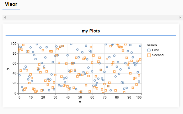
Import tensorflow as tf
# Creating variable for parameter slope (W) with initial value as 0.4
W = tf.Variable([.4], tf.float32)
#Creating variable for parameter bias (b) with initial value as -0.4
b = tf.Variable([-0.4], tf.float32)
# Creating placeholders for providing input or independent variable, denoted by x
x = tf.placeholder(tf.float32)
# Equation of Linear Regression
linear_model = W * x + b
# Initializing all the variables
sess = tf.Session()
init = tf.global_variables_initializer()
sess.run(init)
# Running regression model to calculate the output w.r.t. to provided x values
print(sess.run(linear_model {x: [1, 2, 3, 4]})) 
Below is the implementation for KNN algorithm, the tensorflow way.
import numpy as np
import tensorflow as tf
# Import MINST data
from tensorflow.examples.tutorials.mnist import input_data
mnist = input_data.read_data_sets("/tmp/data/", one_hot=True)
# In this example, we limit mnist data
Xtrain, Ytrain = mnist.train.next_batch(5000) #5000 for training (nn candidates)
Xtest, Ytest = mnist.test.next_batch(200) #200 for testing
# tf Graph Input
xtrain = tf.placeholder("float", [None, 784])
xtest = tf.placeholder("float", [784])
# Nearest Neighbor calculation using L1 Distance
# Calculate L1 Distance
distance = tf.reduce_sum(tf.abs(tf.add(xtrain, tf.negative(xtest))), reduction_indices=1)
# Prediction: Get min distance index (Nearest neighbor)
pred = tf.argmin(distance, 0)
accuracy = 0.
# Initialize the variables (i.e. assign their default value)
init = tf.global_variables_initializer()
# Start training
with tf.Session() as sess:
   sess.run(init)
   # loop over test data
   for i in range(len(Xtest)):
       # Get nearest neighbor
       nn_index = sess.run(pred, feed_dict={xtrain: Xtrain, xtest: Xtest[i, :]})
     # Get nearest neighbor class label and compare it to its true label
       print "Test", i, "Prediction:", np.argmax(Ytrain[nn_index]), \
           "True Class:", np.argmax(Ytest[i])
       # Calculate accuracy
       if np.argmax(Ytrain[nn_index]) == np.argmax(Ytest[i]):
           accuracy += 1./len(Xtest)
   print "Accuracy:", accuracy