Artificial Intelligence: Greedy Best-First Search

Greedy Best-First Search (GBFS) is a heuristic-based search algorithm used in artificial intelligence to find the most promising path from a start node to a goal node in a graph or tree. It prioritizes nodes that appear closest to the goal based on a heuristic function, making it efficient but not always optimal. Below is a detailed explanation:

Key Concepts

• Heuristic Function (h(n)): Estimates the cost from a node $n$ to the goal. For example, in a navigation problem, this could be the straight-line distance to the destination.
• Priority Queue: GBFS uses a priority queue to explore nodes with the lowest heuristic value first.
• Greedy Approach: It selects the node that seems closest to the goal at each step, without considering the total path cost.

Algorithm Steps

1. Initialize:
   • Start with the initial node in the priority queue.
   • Maintain a set of visited nodes to avoid cycles (optional, depending on the problem).
2. Loop:
   • If the queue is empty, return failure (no solution found).
   • Pop the node with the lowest heuristic value$h(n)$.
   • If the node is the goal, return the solution (path).
   • Otherwise, expand the node by generating its neighbors.
   • For each neighbor, compute the heuristic value and add it to the priority queue if not visited.
3. Repeat until the goal is found or the queue is empty.

Greedy Best-First Search for Hierarchical Routing

Step 1: Define the Node Class

Explanation: We create a Node class to represent each node in the graph. The class stores the node’s name and heuristic value, and the __lt__ function allows comparison between nodes based on their heuristic values. This is crucial for maintaining the priority queue.

# Node class to store information about each node
class Node:
    def __init__(self, name, heuristic):
        self.name = name
        self.heuristic = heuristic
    
    def __lt__(self, other):
        return self.heuristic < other.heuristic​

Step 2: Implement Greedy Best-First Search Algorithm

Explanation: This function performs the Greedy Best-First Search algorithm. It starts at the initial node, pushes it onto a priority queue, and explores nodes based on their heuristic values. It first prioritizes nodes within the same region and then moves on to nodes in other regions if necessary.

# Greedy Best-First Search for Hierarchical Routing
def greedy_best_first_search_hierarchical(graph, start, goal, heuristic, region_map):
    priority_queue = []  # Priority queue to hold nodes to explore, sorted by heuristic value
    heapq.heappush(priority_queue, Node(start, heuristic[start]))  # Add start node

    visited = set()  # To keep track of visited nodes
    path = {start: None}  # Path dictionary to track explored paths

    while priority_queue:
        current_node = heapq.heappop(priority_queue).name  # Get node with lowest heuristic

        if current_node == goal:  # Check if goal is reached
            return reconstruct_path(path, start, goal)

        visited.add(current_node)  # Mark current node as visited

        # Explore neighbors in the same region first
        current_region = region_map[current_node]
        for neighbor in graph[current_node]:
            if neighbor not in visited and region_map[neighbor] == current_region:
                heapq.heappush(priority_queue, Node(neighbor, heuristic[neighbor]))
                if neighbor not in path:
                    path[neighbor] = current_node

        # Explore neighbors in other regions
        for neighbor in graph[current_node]:
            if neighbor not in visited and region_map[neighbor] != current_region:
                heapq.heappush(priority_queue, Node(neighbor, heuristic[neighbor]))
                if neighbor not in path:
                    path[neighbor] = current_node

    return None  # If no path is found​

Step 3: Reconstruct the Path

Explanation: Once the goal is reached, this helper function reconstructs the path from the start node to the goal by backtracking through the path dictionary.

# Helper function to reconstruct the path from start to goal
def reconstruct_path(path, start, goal):
    current = goal
    result_path = []
    while current is not None:
        result_path.append(current)  # Add node to path
        current = path[current]  # Move to the parent node
    result_path.reverse()  # Reverse the path to get the correct order
    return result_path​

Step 4: Visualize the Graph and Path

Explanation: This function uses networkx and matplotlib to visually display the graph and highlight the path found by the search algorithm. It also adds labels to the nodes to indicate their region.

# Function to visualize the graph and the path
def visualize_graph(graph, path, pos, region_map):
    G = nx.Graph()

    # Add edges to the graph
    for node, neighbors in graph.items():
        for neighbor in neighbors:
            G.add_edge(node, neighbor)

    plt.figure(figsize=(10, 8))  # Set figure size
    
    # Draw the nodes and edges
    nx.draw(G, pos, with_labels=True, node_size=4000, node_color='skyblue',
            font_size=15, font_weight='bold', edge_color='gray')

    # Highlight the path
    if path:
        path_edges = list(zip(path, path[1:]))
        nx.draw_networkx_edges(G, pos, edgelist=path_edges, edge_color='green', width=3)
        nx.draw_networkx_nodes(G, pos, nodelist=path, node_color='lightgreen')

    # Display region information on the graph
    for node, region in region_map.items():
        plt.text(pos[node][0], pos[node][1] - 0.2, f"Region {region}", fontsize=12, color='black')

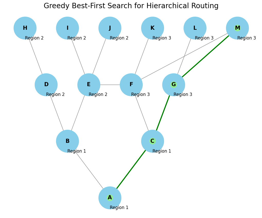
    plt.title("Greedy Best-First Search for Hierarchical Routing", size=20)
    plt.show()​

Step 5: Define the Graph and Heuristic Values

Explanation: We define the graph's structure, where nodes are connected to their neighbors. Additionally, heuristic values for each node and the regions are set to guide the search process.

# Complex graph with hierarchical regions
graph = {
    'A': ['B', 'C'],
    'B': ['D', 'E'],
    'C': ['F', 'G'],
    'D': ['H'],
    'E': ['I', 'J'],
    'F': ['K' , 'M' , 'E'],
    'G': ['L', 'M'],
    'H': [], 'I': [], 'J': [], 'K': [], 'L': [], 'M': []
}

# Heuristic values (assumed for this example)
heuristic = {
    'A': 8, 'B': 6, 'C': 7, 'D': 5, 'E': 4, 'F': 5, 'G': 4,
    'H': 3, 'I': 2, 'J': 1, 'K': 3, 'L': 2, 'M': 1
}

# Define regions for the hierarchical routing (nodes belonging to different regions)
region_map = {
    'A': 1, 'B': 1, 'C': 1, 'D': 2, 'E': 2, 'F': 3, 'G': 3,
    'H': 2, 'I': 2, 'J': 2, 'K': 3, 'L': 3, 'M': 3
}​

Step 6: Execute the Search and Visualize the Result

Explanation: We initiate the Greedy Best-First Search by specifying the start node, goal node, and visualizing the resulting path using the defined graph and heuristics.

# Define positions for better visualization layout (can be modified)
pos = {
    'A': (0, 0), 'B': (-1, 1), 'C': (1, 1), 'D': (-1.5, 2),
    'E': (-0.5, 2), 'F': (0.5, 2), 'G': (1.5, 2), 'H': (-2, 3),
    'I': (-1, 3), 'J': (0, 3), 'K': (1, 3), 'L': (2, 3), 'M': (3, 3)
}

# Perform Greedy Best-First Search for hierarchical routing
start_node = 'A'
goal_node = 'M'
result_path = greedy_best_first_search_hierarchical(graph, start_node, goal_node, heuristic, region_map)

print("Path from {} to {}: {}".format(start_node, goal_node, result_path))

# Visualize the graph and the found path
visualize_graph(graph, result_path, pos, region_map)​

Complete Code: Greedy Best-First Search for Hierarchical Routing

import heapq
import networkx as nx
import matplotlib.pyplot as plt

# Node class to store information about each node
class Node:
    def __init__(self, name, heuristic):
        self.name = name
        self.heuristic = heuristic
    
    def __lt__(self, other):
        return self.heuristic < other.heuristic

# Greedy Best-First Search for Hierarchical Routing
def greedy_best_first_search_hierarchical(graph, start, goal, heuristic, region_map):
    # Priority queue to hold nodes to explore, sorted by heuristic value
    priority_queue = []
    heapq.heappush(priority_queue, Node(start, heuristic[start]))

    visited = set()  # To keep track of visited nodes

    # Path dictionary to track the explored paths
    path = {start: None}

    while priority_queue:
        current_node = heapq.heappop(priority_queue).name

        # If the goal is reached, reconstruct the path
        if current_node == goal:
            return reconstruct_path(path, start, goal)

        visited.add(current_node)

        # Explore neighbors in the same region first, then move to other regions
        current_region = region_map[current_node]
        for neighbor in graph[current_node]:
            if neighbor not in visited and region_map[neighbor] == current_region:
                heapq.heappush(priority_queue, Node(neighbor, heuristic[neighbor]))
                if neighbor not in path:
                    path[neighbor] = current_node

        # Explore neighbors in other regions after same-region neighbors
        for neighbor in graph[current_node]:
            if neighbor not in visited and region_map[neighbor] != current_region:
                heapq.heappush(priority_queue, Node(neighbor, heuristic[neighbor]))
                if neighbor not in path:
                    path[neighbor] = current_node

    return None  # If no path is found

# Helper function to reconstruct the path from start to goal
def reconstruct_path(path, start, goal):
    current = goal
    result_path = []
    while current is not None:
        result_path.append(current)
        current = path[current]
    result_path.reverse()
    return result_path

# Function to visualize the graph and the path
def visualize_graph(graph, path, pos, region_map):
    G = nx.Graph()

    # Add edges to the graph
    for node, neighbors in graph.items():
        for neighbor in neighbors:
            G.add_edge(node, neighbor)

    # Plot the graph
    plt.figure(figsize=(10, 8))
    
    # Draw the nodes and edges
    nx.draw(G, pos, with_labels=True, node_size=4000, node_color='skyblue', font_size=15, font_weight='bold', edge_color='gray')

    # Highlight the path
    if path:
        path_edges = list(zip(path, path[1:]))
        nx.draw_networkx_edges(G, pos, edgelist=path_edges, edge_color='green', width=3)
        nx.draw_networkx_nodes(G, pos, nodelist=path, node_color='lightgreen')

    # Display region information on the graph
    for node, region in region_map.items():
        plt.text(pos[node][0], pos[node][1] - 0.2, f"Region {region}", fontsize=12, color='black')

    plt.title("Greedy Best-First Search for Hierarchical Routing", size=20)
    plt.show()

# Complex graph with hierarchical regions
graph = {
    'A': ['B', 'C'],
    'B': ['D', 'E'],
    'C': ['F', 'G'],
    'D': ['H'],
    'E': ['I', 'J'],
    'F': ['K' , 'M' , 'E'],
    'G': ['L', 'M'],
    'H': [],
    'I': [],
    'J': [],
    'K': [],
    'L': [],
    'M': []
}

# Heuristic values (assumed for this example)
heuristic = {
    'A': 8,
    'B': 6,
    'C': 7,
    'D': 5,
    'E': 4,
    'F': 5,
    'G': 4,
    'H': 3,
    'I': 2,
    'J': 1,
    'K': 3,
    'L': 2,
    'M': 1
}

# Define regions for the hierarchical routing (nodes belonging to different regions)
region_map = {
    'A': 1, 'B': 1, 'C': 1,
    'D': 2, 'E': 2,
    'F': 3, 'G': 3,
    'H': 2, 'I': 2, 'J': 2,
    'K': 3, 'L': 3, 'M': 3
}

# Define positions for better visualization layout (can be modified)
pos = {
    'A': (0, 0),
    'B': (-1, 1),
    'C': (1, 1),
    'D': (-1.5, 2),
    'E': (-0.5, 2),
    'F': (0.5, 2),
    'G': (1.5, 2),
    'H': (-2, 3),
    'I': (-1, 3),
    'J': (0, 3),
    'K': (1, 3),
    'L': (2, 3),
    'M': (3, 3)
}

# Perform Greedy Best-First Search for hierarchical routing
start_node = 'A'
goal_node = 'M'
result_path = greedy_best_first_search_hierarchical(graph, start_node, goal_node, heuristic, region_map)

print("Path from {} to {}: {}".format(start_node, goal_node, result_path))

# Visualize the graph and the found path
visualize_graph(graph, result_path, pos, region_map)​

Output:

Path from A to M: ['A', 'C', 'G', 'M']​

Advantages of Greedy Best-First Search

Limitations of Greedy Best-First Search

Applications of Greedy Best-First Search in AI

Greedy Best-First Search has practical applications across various AI and computer science fields: